1.7183 0 TD 384 316 0.24 -11.24 re W n /TT11 29 0 R f 98 683 1.24 -0.24 re 0.0875 Tw 1.6484 0 TD 0.1672 Tw (worse on five \(AU, ZO, AN, GL, LA\). /TT6 1 Tf ET 0.5195 0 TD Model selection in our context, however, differs in that the)Tj 0.6148 0 TD [( {eibe, ihw}@cs.waikato.ac.nz)]TJ 98 683 0.24 -1.24 re
/TT4 5 0 R 493 377 0.24 -17.24 re 0.6133 0 TD ()Tj f 0.0305 Tw 0.0645 Tc 0.5196 0 TD (S)Tj 0.0513 Tw ()Tj (classification error. ()Tj /TT6 1 Tf )Tj /TT12 1 Tf [(0064 7 856 2889 6026)]TJ 0 Tc 9 0 1.913 9 103 350 Tm 0 Tw ()Tj None of the four considered the use of a resampling)Tj -0.5045 3.4598 TD (Dataset)Tj 0 Tc ()Tj (missing value is added to the coding cost induced by the other branches. 0 Tc 0.0294 Tc ( 2.41:)Tj 441 404 0.24 -1.24 re -0.0006 Tc )Tj (Comparing the tree sizes produced by the same two methods, one might expect E-)Tj 0.105 Tc
0 Tc 241.52 201.96 m /GS1 6 0 R 276 220 0.24 -11.24 re 198 266 168 -84 re ( [1.51874,1.5201\) : 1 \(5\))Tj 18 0 0 18 195.7812 543.4687 Tm (ad hoc)Tj 0.6148 0 TD 275.437 397.469 m 0 -1.8333 TD f ()Tj T* -0.0286 Tc The fourth, GR, was chosen)Tj By the end of this course you should be able to: 263 404 0.24 -1.24 re << ()Tj f 217.52 201.96 m /TT16 1 Tf 5.3878 0 TD (techniques. 8.6667 0 TD [(L)175.3(Y)-5713.3(48.0)]TJ (Al )Tj ()Tj -0.5391 0.013 TD f 20 0 obj 439 362 53.24 -0.24 re
 (node during construction of a decision tree, rather than applying it to the finished)Tj /TT12 1 Tf -18.2355 -1.0833 TD /TT4 1 Tf ET 7 0 0 7 111.5625 561 Tm -2.4013 -1 TD 166 266 0.24 -11.24 re 5.3878 0 TD 0.0639 Tc 0.1505 Tw 12 0 0 12 293 39 Tm 301.48 215.484 304.392 217.5 307.98 217.5 c (problem, the appropriate attribute at each node being determined by comparing the)Tj /TT12 1 Tf <0027>Tj /TT4 1 Tf 0 Tc (E-CV)Tj 0.0645 Tc f 440 607 0.24 -11.24 re
 167 362 55.24 -0.24 re /TT4 1 Tf >> 0.68 0 TD 0.0278 Tc (In contrast to T2, we allow nodes corresponding to a missing-value branch to be)Tj /TT11 1 Tf f 0.0164 Tw ( is the number of members of the test set )Tj (| | | | | | | Mg )Tj [(0.2)-2489.7(7.5)]TJ [(1.1)-2489.7(5.2)]TJ /Font << /TT4 5 0 R 12 0 0 12 480 209 Tm /TT16 1 Tf )Tj 0 -1.8333 TD /TT17 1 Tf 0 0.5703 TD /TT12 1 Tf 207.432 212.46 204.52 214.476 204.52 216.96 c ()Tj )Tj 276 362 0.24 -17.24 re 0.0833 Tc f f (L)Tj -0.0293 Tc 0.5188 0 TD 0.0117 Tc -0.0072 Tc 0.6133 0 TD BT /TT4 5 0 R 0 Tc 0.6133 0 TD (=)Tj [(1.0)-1935.5(19.6)]TJ 5.3867 0 TD f -0.0074 Tc f /Length 16864 0.4438 0 TD -4.4954 -1.0833 TD 246.5 220.25 m 0.5195 0 TD 0 -1.0833 TD (. ET 0.0927 Tc This makes them easier to)Tj 0 Tw f (significantly change the accuracy of the resulting tree; moreover, it does not address)Tj /TT16 1 Tf (validation, GR )Tj /TT4 1 Tf 0.0131 Tc W n 0.0024 Tc /TT11 1 Tf T* f BT 0 Tc 0 Tw ()Tj /TT4 1 Tf ET T* /TT6 1 Tf 332 617 0.24 -11.24 re S 0.6133 0 TD /TT11 29 0 R -0.0142 Tc 262 225 34 -23 re 0.6113 0 TD (and this is what we employed \(we also used the bootstrap method, and it gave)Tj T* 0.003 Tc (=)Tj ()Tj /TT4 1 Tf 493 351 0.24 -11.24 re 494 577 0.24 -17.24 re 1.7297 0 TD [(C)64.5(R)-5934.8(16.4)]TJ /TT4 1 Tf Cut to a certain depth: The tree may have overfit the training data and build an overly complex model. 28 0 obj 0.0202 Tw 98 346 0.24 -11.24 re [(they send more than 50% of training instances directly to leaf nodes. /TT12 1 Tf /ProcSet [/PDF /Text ] These methods are called resampling)Tj /TT12 1 Tf 0.2283 Tw 371.5 199.524 374.412 201.54 378 201.54 c -0.0077 Tc f T* T* 0 Tc (C)Tj 0.0058 Tc 6.2971 0 TD /TT12 30 0 R Then, for nodes which transfer)Tj 0.0062 Tw Analytics Vidhya is a community of Analytics and Data Science professionals. [(1.0)-1934.9(14.3)]TJ <0044>Tj (log)Tj /TT6 1 Tf /TT4 1 Tf 263 311 0.24 -11.24 re T* 98 597 0.24 -11.24 re 0.0743 Tw /TT4 1 Tf 207 404 1.24 -0.24 re /TT16 1 Tf ()Tj 0.6133 0 TD -2.3984 -1 TD -0.0047 Tc 0.1445 Tw -0.0024 Tc T* /TT16 1 Tf 0.0645 Tc & Ron, D. \(1995\): An Experimental and)Tj 0.091 Tw 384 326 0.24 -11.24 re 0.0091 Tc f 330 210 0.24 -11.24 re /TT4 1 Tf 0.0323 Tw -1.2057 -2.9818 TD Consequently, instead of using a resampling estimate of the)Tj )]TJ (., 1995\).
0.0969 Tw (k)Tj f 442 189 51.24 -0.24 re 0 Tc /TT4 1 Tf 5.3878 0 TD (et al)Tj 3 0 TD )Tj 12 0 0 12 290 39 Tm /TT4 1 Tf (call for new model selection methods. /TT6 1 Tf 0 0 0 rg ( [1.5201,+)Tj /TT17 1 Tf 0.0015 Tc 153 259 277.24 -0.24 re -2.399 -1 TD 0.0264 Tw 492 286 0.24 -11.24 re /TT16 1 Tf (Attribute 2)Tj (structure of such models. 10.8354 0 TD 190.824 206.96 193.96 204.72 193.96 201.96 c
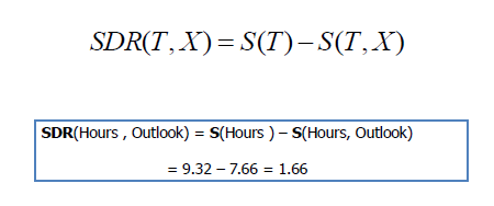
520 700 0.24 -399.24 re 12 0 0 12 132.3125 689 Tm \(p_c\) is the proportion of samples in category \(c\). >> )Tj ET -20.5014 -1 TD /TT17 1 Tf
(ad hoc)Tj Since this process is essentially a recursive segmentation, this approach is also called recursive partitioning. (k)Tj 30.0075 0 TD 0.0915 Tw q >>
-0.0084 Tc 179 234 64 -38 re
/TT6 1 Tf For this we use:)Tj
0 Tc 0.6148 0 TD 9 0 0 9 112 204 Tm (number in order to obtain small, accurate trees. 330 379 1.24 -0.24 re 440 700 0.24 -17.24 re 0 Tw (S)Tj (Quinlan, R. \(1993\): )Tj 0.6133 0 TD (2.3)Tj 9 0 0 9 112 512 Tm 21.8302 0 TD ( 1.51838: 1 \(36.0/3.8\))Tj 0 Tc 5.9423 0 TD -6.0193 -1.0833 TD 0 Tc (0.4)Tj However, the recursive situation differs from the usual one, and may)Tj -2.25 -1.8333 TD /TT16 1 Tf (entropy-based rather than an error-based measure is central to this paper. 12 0 0 12 289 253 Tm 438 379 1.24 -0.24 re 379.25 192 l 0.0833 Tc ET /TT4 1 Tf 0.0645 Tc f /TT4 1 Tf -0.0053 Tc (\(because no prepruning is applied\)indeed, it produces considerably smaller trees)Tj /TT17 1 Tf (error-based criterion. -0.0029 Tc 12 0 0 12 293 39 Tm [(1.2)-1935.5(80.7)]TJ (| | | Na )Tj 219 521 0.24 -11.24 re /TT12 1 Tf 263 281 0.24 -11.24 re
T* -26.8523 -1.0833 TD 0.0652 Tc
440 497 1.24 -0.24 re 98 301 1.24 -0.24 re /StemH 139 (CV to build smaller trees since the set of potential split points for the classification)Tj /ProcSet [/PDF /Text ] -0.0293 Tc (k )Tj
-0.0274 Tc (its lack of stability: for some datasets it produces results with much lower accuracy. 0.681 0 TD 0.0025 Tc /TT6 1 Tf -0.0018 Tc 1.7276 0 TD /Length 70 0.0002 Tc -0.0045 Tc
(Selecting Multiway Splits in Decision Trees)Tj /GS1 6 0 R 0.6133 0 TD 492 306 0.24 -11.24 re (Al )Tj 59 0 obj 0 -1.0833 TD 3.4816 0 TD /ExtGState << (. ()Tj /TT4 1 Tf 0 g /TT12 1 Tf stream ( since that is not necessary to minimize the classification error. [(error. ()Tj ET 0.0297 Tw 0.0259 Tc (multiway split on a numeric attribute that incorporates the decision of how many)Tj f 5.3867 0 TD q 0.6133 0 TD ( 1.5186: 2 \(5.0/1.2\))Tj -0.0293 Tc T* The hands-on section of this course focuses on using best practices for classification, including train and test splits, and handling data sets with unbalanced classes. 0 Tc /TT6 1 Tf 386 511 0.24 -14.24 re 0 Tc 263 361 0.24 -11.24 re 0 Tc 0.1078 Tw (An argument, illustrated in Figure 1, was presented above for the use of)Tj /TT16 1 Tf -4.6868 -1 TD [(1.6)-1935.5(63.8)]TJ (| | | | Mg )Tj -0.0299 Tc /TT16 1 Tf -0.0025 Tc 0 Tc [(A)176.9(N)-6489.7(0.6)]TJ
276 190 0.24 -14.24 re <0029>Tj 0.0166 Tw 0 Tw /TT2 1 Tf BT 6.461 0 TD 0 -1.7214 TD 222 266 0.24 -11.24 re -0.0069 Tc )Tj /TT4 1 Tf 0 Tc /TT11 1 Tf (1.8)Tj 372.469 392 l /TT17 1 Tf (\(\))Tj /TT4 1 Tf -13.5572 -1.0833 TD 0.6133 0 TD (Ba > 0.27:)Tj f -0.0288 Tc 381 213 0.24 -11.24 re BT 263 351 0.24 -11.24 re -0.0061 Tc 0.0011 Tc 492 326 0.24 -11.24 re ET 0.0121 Tc [(0.7)-1935.5(14.1)]TJ (1.3)Tj 0 Tc -0.0268 Tc -0.0292 Tc T* 0.0362 Tc ()Tj T* 0.0105 Tw -0.003 Tc 0.0178 Tc
/TT4 1 Tf f -0.0024 Tc 0.0039 Tc -0.0268 Tc 2.8125 0.763 TD 492 346 0.24 -11.24 re 0 Tw f (branch by one generated using E-CV. (The gain ratio evaluation of a )Tj -0.005 Tc An)Tj However, we found that this modification did not)Tj 12 0 0 12 298.0665 551 Tm ( 13.75: 2 \(3.0/1.1\))Tj ()Tj 441 700 53.24 -0.24 re 0.6133 0 TD f (better decision tree because a secondary split will be made on the other attribute. 163 511 0.24 -14.24 re 219 561 0.24 -11.24 re 0.1113 Tc (th subinterval)Tj 0.0645 Tc (The multiway split consists of the intervals corresponding to this trees leaves. In the two-class case its accuracy is significantly higher for three datasets \(CR,)Tj 152 259 0.24 -83.24 re f /TT2 1 Tf 0.6902 0 TD 0 Tc S /TT16 1 Tf 12 0 0 12 270.6563 252.8438 Tm 9 0 0 9 112 608 Tm /TT4 1 Tf [(2.9)-1936(78.4)]TJ T* /TT12 1 Tf /ProcSet [/PDF /Text ] 0.4316 0 TD f /TT4 1 Tf 0.5 w S 263 377 0.24 -17.24 re (arises whenever attributes with different numbers of branches are compared. 5.3867 0 TD /TT17 1 Tf (Ba )Tj 0.6122 0 TD 14.174 0 TD 0 Tw 4.8267 0 TD 0 Tc 0 Tc BT 0.5196 0 TD -0.0073 Tc 0.6133 0 TD
ET f [(1.5)-1935.5(29.0)]TJ 330 379 0.24 -1.24 re (attributes in a decision tree. 219 511 0.24 -14.24 re T* 1.3626 Tc [(0.6)-1935.5(28.3)]TJ ()Tj -4.1035 -1.0833 TD -1.8151 1.6328 TD
/TT11 1 Tf -0.0287 Tc /TT4 1 Tf 1 g 5.3867 0 TD f (Continuous Features, )Tj ( replaced by)Tj f [(,)-333.3(\(3\))]TJ 0.75 g /TT4 1 Tf 0.6133 0 TD -3.0964 -2.2187 TD /TT4 1 Tf /TT16 1 Tf 0 Tc (Construction, )Tj (\) : 1 \(15/2\))Tj 0.067 Tw f 0.1155 Tw 4.0067 0 TD (\))Tj -4.616 -1.0833 TD 0 Tw 0 Tc /TT12 1 Tf
0.6133 0 TD T* 0 Tw f f [(2.7)-1935.5(93.2)]TJ
(multiway split is used directly to classify instances, and should therefore be)Tj (| | K > 0.03:)Tj f 5.3867 0 TD 17.4643 0.0045 TD 0 Tc 0.106 Tw ET /TT17 1 Tf 311.844 218 314.98 215.76 314.98 213 c 0 Tc T* on Artificial Neural Networks and Expert Systems)Tj If we were to classify everything as either 1, or 0, which is what we're doing with each one of our subsets, using that majority class. (of terminating growth by pre-pruning. 0 -1.8333 TD
-18.4592 -1.0833 TD 0 Tc 5.3867 0 TD [(1.6)-1935.5(24.8)]TJ 163 597 0.24 -11.24 re 0 Tw -0.0304 Tc /TT4 1 Tf 354.25 185.75 l T* -0.0295 Tc f f (minimum description length formula for multi-split selection, I-CV )Tj
ET <0029>Tj stream 189.031 549.281 l <003c>Tj 0.0069 Tc /TT4 1 Tf 0 Tc [(1.3)-1934.9(12.2)]TJ 56 0 obj 0 Tw 0.1505 Tw 5.3867 0 TD
/TT4 1 Tf f 6.0156 0.7135 TD (| | | | | | RI > 1.51629: 2 \(2.0/1.0\))Tj f BT /TT4 1 Tf ET [(1.6)-2490.3(3.8)]TJ /TT6 1 Tf 0.0106 Tc /TT12 1 Tf 0.0645 Tc 1 i (more comprehensible than the usual binary trees because attributes rarely appear)Tj Joint Conf. ET Q 5.3307 0 TD ( examples to be covered by)Tj 0 0 0 rg )Tj f [(1.1)-1935.5(23.7)]TJ f 0 Tc 0 g -0.0295 Tc 0 g 0 Tc 1 i (Several algorithms for finding the optimal multiway split on a numeric attribute)Tj