It should be easy if required data can be pulled exactly.
The =LEN formula is an Excel function that allows you to find out the number of text characters in a cell. Save yourself hours of learning and, more importantly, hard work from using Excel formulas, and make your life easier with a more efficient, secure and precise automated PIM system. The. One way to keep your product inventory in order and save time when locating, adding and editing data is to use formulas that provide shortcuts for finding and combining data, as well as extracting analysis conclusions. The calculation of the planned production cost price begins with the determination of the production cost of raw materials and materials used for the production of goods (which are directly involved in the technological process). Because the intention is to calculate the average of fuel consumption per car not per trip. By clicking Post Your Answer, you agree to our terms of service, privacy policy and cookie policy. Is there a suffix that means "like", or "resembling"? SUMIFS supports logical operators (>, Formulas are the key to getting things done in Excel.In this accelerated training, you'll learn how to use formulas to manipulate text, work with dates and times, lookup values with VLOOKUP and INDEX & MATCH, count and sum with criteria, dynamically rank values, and create dynamic ranges.
This shortcut is useful for identifying different types of product codes according to their length.
We get a lower safety stock value (and so a lower Reorder Point value) than in the previous case because in this example the lead time variation is rather small.This method can be used if the demand uncertainty is negligible compared to the lead time variation. Select B2. For example, 2 quarts of paint are used to produce one piece of a finished good, and the paint is picked in 25-quart cans. The last column - the planned production cost factor - will show the level of costs that the company will incur for the delivery of products.
These data can be taken in the technological or production department.
The following method assumes a normal distribution of demand (also called the Kings method).
I need help to come out with a solution for this: Actually I want to calculate my electricity consumption. We can't guess what needs to be done given only what you have so far. If you hold unnecessary stock levels to cover all those issues, you will have unreasonably high stock costs. This is an average of, Over 12 months, we had 10 deliveries. =CONCATENATE enables you to combine different types of data (numbers, text, dates) in one single cell. Follow these easy steps to disable AdBlock, Follow these easy steps to disable AdBlock Plus, Follow these easy steps to disable uBlock Origin, Follow these easy steps to disable uBlock. First, you must consider outliers values: if you have an extreme lead time or sale value once in your past data, this will give you very high safety stock. You dont want to use this value in the calculation, as it doesnt reflect your regular business: you dont want to cover such high uncertainty.Then, even if you exclude outliers, you will always cover the most extreme case: it means you will have high stock levels the whole year, and thus high inventory costs. We make the assumption that what happened in the past will repeat itself: if we protect against the most extreme case (the highest supply variation combined with the highest demand variation) then we are sure to cover any future risk.This is the average max method that I also call the prudent father method.Safety Stock formula: SS = (Max Lead Time Max Sale) (Average Lead time Average Sale). And what you actually need to calculate - cost? How to calculate value based on cell row in Excel? There are still other methods for calculating the safety stock, that can solve the problem of demand and lead time that are not normally distributed: If you already have a good understanding of Safety Stock, Reorder calculations and statistics, you can add a bit more complexity by trying those methods.
Keep in mind that data quality is more important than the method. Before considering the formulas, I would like to stress the risks involved in safety stock.
How to combine data and calculate in Excel with formula, Calculate Distinct Values Based On 4 Conditions (Excel Formula), Creating an excel formula to calculate returns, Excel formula to calculate based on another field's contents, Calculate average annual growth rate per group in excel, Existence of a negative eigenvalues for a certain symmetric matrix.
the first consumption 0-200kwh, rate $0.218, for 201-300 consumption rate is $0.334, 301-600 rate is $0.516, 601-900 rate is $0.546.
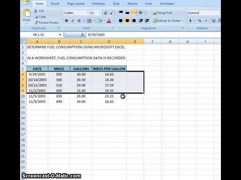
You must record required data every time you refuels your car. From experience, you know that owning 5 days of supplies is enough to mitigate supply and demand risks.Safety Stock formula and Calculation: So your safety stock is simply 100 5 = 500 pieces. In the first case, we will only consider uncertainty about the demand. This article provides information about various options that are related to the calculation of material consumption. For a better experience, please enable JavaScript in your browser before proceeding. I never miss watching NBA finals, Tennis Grand Slam Finals, Formula 1, MotoGP, football tournaments and competitions. The fixed consumed quantity can be set up in intervals of the produced quantity. This function is important for when you need to perform operations in Excel that require numeric values. In fact - the purchase price, issued by the supplier; transportation expenses for the delivery of goods to the warehouse; duty and customs fees, if we import goods from abroad. The first refueling average value is calculated by subtracting odometer value from 2nd row with 1st row from refueling table.
Any calculation must contain a decoding of the costs of materials and wages. In the column Amount the formula works: = D3 * E3. Hello, I have a file that I use to track a unit forecast. As a result, you can track which trip that cause your car to consume more fuel than usual. It doesnt consider any seasonality (if you have a forecast that takes into account the seasonality, you can use it with the corresponding deviation). There is also a complementary formula if you just want to obtain the number of working days between two dates: This formula will show you the minimum figure from a set of values, such as the lowest purchase or sales price for a product.
You have low volumes: try the average min/max method. There are three big parts in this one worksheet where you need to pay attention. Here are a few tips for choosing a method: I recommend you to check out our videos tutorial : If you want to go to the next level, join my next Inventory Management Workshop (free): How to avoid shortages and overstocks in times of great uncertainty. The key to this approach is to use Excel Tables, because Table ranges automatically expand to handle changes in data.
After all, enterprises bear different costs depending on the type of activity.
Whatever the method used, there are limitations: I recommend using a service rate target based on a classification.
The normal distribution is a probability distribution symmetric to the mean.
We can then combine EOQ with Safety Stock to ensure optimized ordering quantities and protection against uncertainty.
Then, it is divide by purchased volume from 1st row.
Are shrivelled chilis safe to eat and process into chili flakes? You might have a stronger safety stock on the umbrella to cover higher risks of shortages. Be the first to rate this template.
 The average lead time is 1.15 months.To get the safety stock quantity, we need to multiply the service factor Z by the demand standard deviation and the square root of the lead time L. We get a Safety Stock level of 194 pieces. as the attached pic. You need a safety stock to cover yourself against two hazards or uncertainties: demand and lead time. Safety stock can be reassuring, but it often reflects fundamental problems: poor data accuracy, poor forecast accuracy, outdated IT systems, lack of communication with suppliers Typically, maintaining high safety stock is a trick to hide the root causes of our issues. Nowadays, most of cars are equipped with electronic device that will display its fuel consumption in real time. How to choose the right formula for your Safety Stock?
 Here we have a Reorder point of 1578 units.This method has the advantage to be very simple to implement. These are other basic formulas for browsing your inventory in Excel, particularly useful if you have a lot of products or SKUs. You dont have any data about lead time (or unreliable data): this is common. SUMIFS is a function to sum cells that meet multiple criteria. The basic Safety Stock scenario follows a Continuous Review Policy: quantities to order are fixed.
It would be different if we used a forecast). This will prevent any disparities between the numbers from your sales channels and your actual inventory, and will allow you to manage your stock level appropriately. They are used to show you the value comparison between the first and the last four refueling trip. As an alternative to nested IF() you may want to consider a lookup table sorted by the consumption threshold values. You have higher volumes: use the normal distribution method.
To make it more convenient to set percentages, we sort the data by the column Name of product. Note! Track your performance and adjust (see next the Action Plan I recommend). For example, you can use it to find out the yearly net profit provided by a product by using its code cell.
If you use the default value, Standard, the consumption isn't calculated from a formula.
We will go through 6 calculation methods for your safety stock, from the simplest to the most complex one. Get over 100 Excel Functions you should know in one handy PDF. This function allows you to delete content from a cell. MRP: Materials Planning Model: Formula suggestion needed (Run out Date of Materials), How to calculate fuel consumption in Excel, Need help with formula to calculate materials, I am looking for help developing a formula to calculate utility consumption, How to calculate my inventory days when I have the consumption Data.
Its essential to manage the number of units for each product that comes into your inventory. We take a certain group of goods. Only in this case the program will calculate correctly. It is better to learn how to calculate the production cost price from the sphere of trade. Remember that the goal is to balance inventory costs and customer service rate. With this formula you can calculate the number of days between certain dates in cells.
Here is the calculation: It's assumed that 0.5 meter of tube is scrapped for every five pieces of tube that are consumed.
They are not giving you information of your single trip, except you reset the odometer every time you go. If A2:A50000 contain data. Knowing the norms, we can calculate the cost of materials (the calculation is for thousands of items): In this table, you have to manually fill in only one column Price.
I'd also add typing in all caps is considered internet impolite, Hi, sorry for the caps, no intention to impolite.huhuu. Try method 3 or 5 first, depending on your data.
(Height * Width * Depth / Density) * Constant, Number of multiples that are required for 10 pieces of the finished good: 10 2 = 5 pieces, Total consumption: 4.5 5 = 22.5 meters of metal tube, Paint that is required, excluding scrap: 180 2 = 360 quarts, Number of cans: 360 25 = 14.4, which is rounded up to 15, Paint that is required, including scrap: 15 25 = 375 quarts. Either it is for your own private purposes or company purposes.
For example, lets say your supplier had an exceptional issue, and one of your shipments had very high lead time. 2020 - All rights reserved, Fuel consumption spreadsheet is not correct. This means we can get a total of all incoming red items with: And a total of all outgoing red items with: In both cases, the SUMIFS function generates a total for all red items in each table.